

| Citation: |
Lea Safetly, Toni Sayah. ON THE INVERSE PROBLEM FOR THE BURGERS' EQUATION WITH SMOOTH INITIAL DATA IN A BOUNDED DOMAIN[J]. Journal of Applied Analysis & Computation, 2027, 17(2): 1014-1037. doi: 10.11948/20260119

|
ON THE INVERSE PROBLEM FOR THE BURGERS' EQUATION WITH SMOOTH INITIAL DATA IN A BOUNDED DOMAIN
-
Abstract
In this paper, we study the inverse problem of recovering smooth initial data for the one-dimensional Burgers' equation on a bounded spatial domain. Specifically, this problem focuses on recovering the initial condition from measurements at a part of the boundary over a given time interval. We therefore prove the uniqueness of the solution to the direct problem and establish, under certain assumptions, a stability estimate for the inverse problem based on a backward method in time and space, showing that the initial data can be reconstructed in this smooth case. To validate our theoretical results, we perform several numerical simulations and demonstrate the effectiveness of the proposed approaches.
-

-
References
[1] O. M. Alifanov, Inverse Heat Transfer Problems, Springer-Verlag, Berlin, 1994. [2] L. Ambrosio, Transport equation and Cauchy problem for BV vector fields, Inventiones Mathematicae, 2004, 158(2), 227–260. doi: 10.1007/s00222-004-0367-2 [3] K. Ammar, P. Wittbold and J. Carrillo, Scalar conservation laws with general boundary condition and continuous flux function, Journal of Differential Equations, 2006, 228(1), 111–139. doi: 10.1016/j.jde.2006.05.002 [4] C. Bardos, A. Y. Leroux and J. C. Nedelec, First order quasilinear equations with boundary conditions, Communications in Partial Differential Equations, 1979, 4(9), 1017–1034. doi: 10.1080/03605307908820117 [5] H. Bateman, Some recent researches on the motion of fluids, Monthly Weather Review, 1915, 43(4), 163–170. doi: 10.1175/1520-0493(1915)43<163:SRROTM>2.0.CO;2 [6] J. V. Beck, B. Blackwell and C. R. St. Clair, Inverse Heat Conduction: Ill-Posed Problems, Wiley-Interscience, New York, 1985. [7] F. Boyer, Trace theorems and spatial continuity properties for the solutions of the transport equation, Differential and Integral Equations, 2005, 18(8), 891–934. [8] F. Boyer, Analysis of the upwind finite volume method for general initial- and boundary-value transport problems, IMA Journal of Numerical Analysis, 2012, 32(4), 1404–1439. doi: 10.1093/imanum/drr031 [9] J. M. Burgers, A mathematical model illustrating the theory of turbulence, Advances in Applied Mechanics, 1948, 1, 171–199. [10] C. Castro, F. Palacios and E. Zuazua, Optimal control and vanishing viscosity for the Burgers equation, in Integral Methods in Science and Engineering, Volume 2, Birkhäuser, Boston, 2010, 65–90. [11] P. Colella, Multidimensional upwind methods for hyperbolic conservation laws, Journal of Computational Physics, 1990, 87(1), 171–200. doi: 10.1016/0021-9991(90)90233-Q [12] R. J. DiPerna and P. L. Lions, Ordinary differential equations, transport theory and Sobolev spaces, Inventiones Mathematicae, 1989, 98(3), 511–547. doi: 10.1007/BF01393835 [13] F. Dubois and P. G. LeFloch, Boundary conditions for nonlinear hyperbolic systems of conservation laws, Journal of Differential Equations, 1988, 71(1), 93–122. doi: 10.1016/0022-0396(88)90040-X [14] L. C. Evans, Partial Differential Equations, 2nd ed., American Mathematical Society, Providence, Rhode Island, 2010. [15] E. Godlewski and P. -A. Raviart, Hyperbolic Systems of Conservation Laws, Ellipses, Paris, 1991. [16] S. K. Godunov, A difference method for numerical calculation of discontinuous solutions of the equations of hydrodynamics, Matematicheskii Sbornik, 1959, 47(89), 271–306. [17] L. Gosse and E. Zuazua, Filtered gradient algorithms for inverse design problems of one-dimensional Burgers equation, in Innovative Algorithms and Analysis, Springer International Publishing, 2017, 197–227. [18] A. Harten, High resolution schemes for hyperbolic conservation laws, Journal of Computational Physics, 1983, 49(3), 357–393. [19] V. Isakov, Inverse Problems for Partial Differential Equations, 2nd ed., Springer, New York, 2006. [20] M. T. Jenaliyev, S. I. Kabanikhin, M. Kassen and M. G. Yergaliyev, On the solvability of an inverse problem for the Burgers equation with an integral overdetermination condition in a nonlinearly degenerating domain, Journal of Inverse and Ill-Posed Problems, 2025, 33(1), 24–41. [21] S. I. Kabanikhin, Definitions and examples of inverse and ill-posed problems, Journal of Inverse and Ill-Posed Problems, 2008, 16(4), 317–357. [22] M. M. Lavrent'ev, V. G. Romanov and S. P. Shishatskii, Ill-Posed Problems of Mathematical Physics and Analysis, Translations of Mathematical Monographs, Vol. 64, American Mathematical Society, Providence, Rhode Island, 1986. [23] P. G. LeFloch, Hyperbolic Systems of Conservation Laws: The Theory of Classical and Nonclassical Shock Waves, Birkhäuser, Basel, 2002. [24] R. J. LeVeque, Numerical Methods for Conservation Laws, 2nd ed., Birkhäuser, Basel, 1992. [25] R. J. LeVeque, Finite Volume Methods for Hyperbolic Problems, Cambridge University Press, Cambridge, 2002. [26] T. Liard and E. Zuazua, Analysis and numerical solvability of backward-forward conservation laws, SIAM Journal on Mathematical Analysis, 2023, 55(3), 1949–1968. doi: 10.1137/22M1478720 [27] T. Liard and E. Zuazua, Initial data identification for the one-dimensional Burgers equation, IEEE Transactions on Automatic Control, 2022, 67(6), 3098–3104. doi: 10.1109/TAC.2021.3096921 [28] D. Lukyanenko, T. Yeleskina, I. Prigorniy, T. Isaev, A. Borzunov and M. Shishlenin, Restoring the initial condition in the inverse problem for a nonlinear equation of the reaction–diffusion–advection type with data on the position of a reaction front measured with a time delay, Mathematics, 2021, 9(4), 342. [29] S. Mishra, U. S. Fjordholm and R. Abgrall, Numerical Methods for Conservation Laws and Related Equations, Lecture Notes, 2019. [30] L. C. M. Pereira, B. A. Carmo, M. A. Rincón and R. F. Apolaya, Theoretical and numerical study of a Burgers viscous equation type with moving boundary, Mathematical Methods in the Applied Sciences, 2025, 48(4), 5255–5277. [31] J. Qin, Y. Meng and S. Yi, Optimal control of the inverse problem of the Burgers equation for representing the state of sonic vibration velocity in water, Mathematics, 2024, 12(22), 3625. [32] J. Qin, J. Zhao, J. Xu and S. Yi, Optimal control of the inverse problem of the fractional Burgers equation, Fractal and Fractional, 2025, 9(8), 484. [33] L. Safetly, T. Sayah and F. Triki, Inverse problem for Burgers' equation: Recovering Riemann initial data, Applicable Analysis, 2026, 105(12), 2616–2661. [34] E. F. Toro, Riemann Solvers and Numerical Methods for Fluid Dynamics: A Practical Introduction, 3rd ed., Springer, Berlin, 2009. [35] T. Voy, One Dimensional Burgers Equation, Department of Applied Mathematics, Gran Sasso Science Institute, L'Aquila, Italy, 2018. -
-
Figures(26)

Export File
Citation
Lea Safetly, Toni Sayah. ON THE INVERSE PROBLEM FOR THE BURGERS' EQUATION WITH SMOOTH INITIAL DATA IN A BOUNDED DOMAIN[J]. Journal of Applied Analysis & Computation, 2027, 17(2): 1014-1037. doi: 10.11948/20260119
Format
Content
 DownLoad:
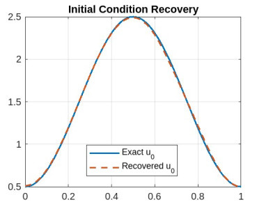
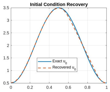
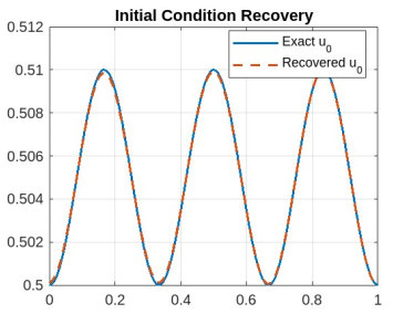
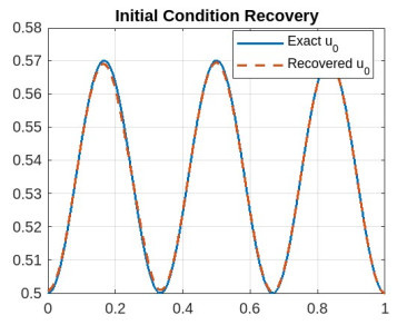
-
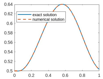
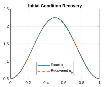
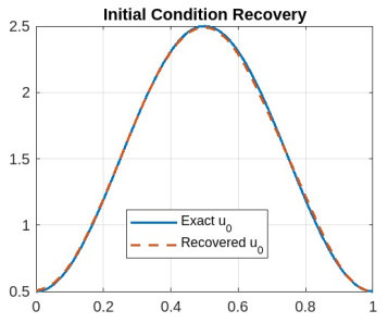
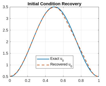
Figure 1.
Comparison of the exact and numerical solution for
$ t=0.1 $ -
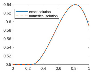
Figure 2.
Comparison of the exact and numerical solution for t = 0.5.
-
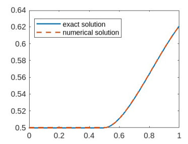
Figure 3.
Comparison of the exact and numerical solution for t = 1.
-
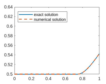
Figure 4.
Comparison of the exact and numerical solution for t = 1.5.
-
Figure 5.
Comparison between exact and recovered initial data for b = 0.14.
-
Figure 6.
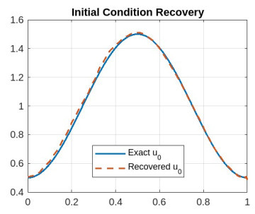
Comparison between exact and recovered initial data for b = 10.
-
Figure 7.
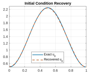
Comparison between reconstructed and exact initial condition for m = 1 and b = 1.5.
-
Figure 8.
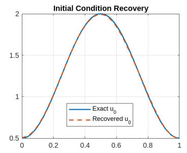
Comparison between reconstructed and exact initial condition for m = 1 and b = 1.75.
-
Figure 9.
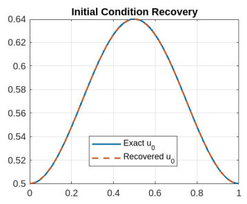
Comparison between reconstructed and exact initial condition for m = 1 and b = 2.
-
Figure 10.
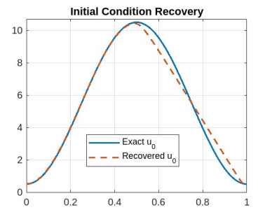
Comparison between reconstructed and exact initial condition for m = 1 and b = 3.
-
Figure 11.
Comparison between reconstructed and exact initial condition for m = 3 and b = 0.01.
-
Figure 12.
Comparison between reconstructed and exact initial condition for m = 3 and b = 0.07.
-
Figure 13.
Comparison between reconstructed and exact initial condition for m = 3 and b = 0.15.
-
Figure 14.
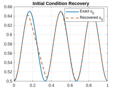
Comparison of the exact and reconstructed initial conditions u0 with white noise on u at x = 1, for α = 0.1, m = 1 and b = 1.
-
Figure 15.
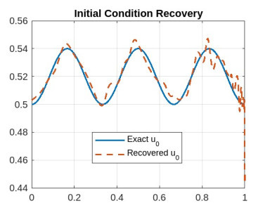
Comparison of the exact and reconstructed initial conditions u0 with white noise on u at x = 1, for α = 0.1, m = 3 and b = 0.04.
-
Figure 16.
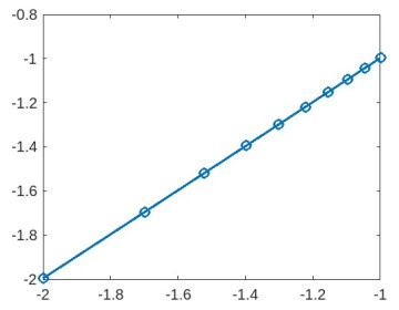
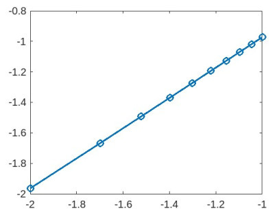
Variation of log10(e2j) with respect to log10(e1j), for m = 1 and b = 1.
-
Figure 17.
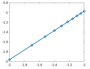
Variation of log10(e2j) with respect to log10(e1j), for m = 3 and b = 0.04.
-
Figure 18.
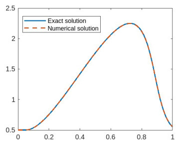
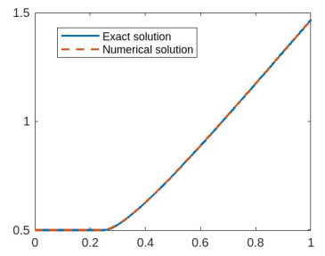
Comparison between the exact and numerical solution for m = 1 and b = 1.75.
-
Figure 19.
Comparison between the exact and numerical solution for m = 1 and b = 1.75.
-
Figure 20.
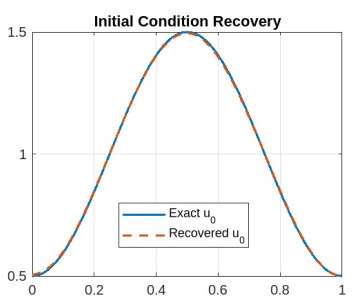
Comparison between the recovered and exact initial data for m = 1 and b = 1.
-
Figure 21.
Comparison between the recovered and exact initial data for m = 1 and b = 1.75.
-
Figure 22.
Comparison between the recovered and exact initial data for m = 1 and b = 2.
-
Figure 23.
Comparison between the recovered and exact initial data for m = 1 and b = 3.
-
Figure 24.
Variation of log10(e2j) with respect to log10(e1j), for m = 1 and b = 1.
-
Figure 25.
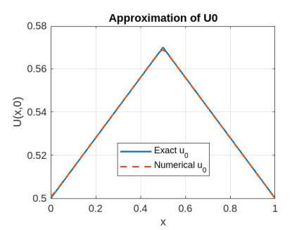
Comparison between exact and numerical initial data for b = 1.75.
-
Figure 26.
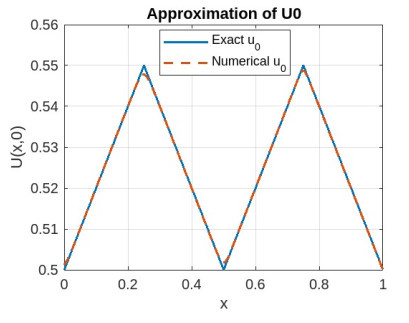
Comparison between exact and numerical initial data for b = 0.05.